RNA-Seq data analysis

RNA-Seq computational approach tutorial approachs.

Pipeline

Introduction

RNA-Seq (RNA sequencing ) also called whole transcriptome sequncing use next-generation sequeincing (NGS) to reveal the presence and quantity of RNA in a biolgical sample at a given moment. RNA-seq produces millions of sequences from complex RNA samples. With this powerful approach, you can:

Measure gene expression.
Discover and annotate complete transcripts.
Characterize alternative splicing and polyadenylation.

The RNA-seqlopedia provides an overview of RNA-seq and of the choices necessary to carry out a successful RNA-seq experiment.

In this tutorial we will try different practical analisys of RNA-seq:

Counting methods
Pseudomapping methods

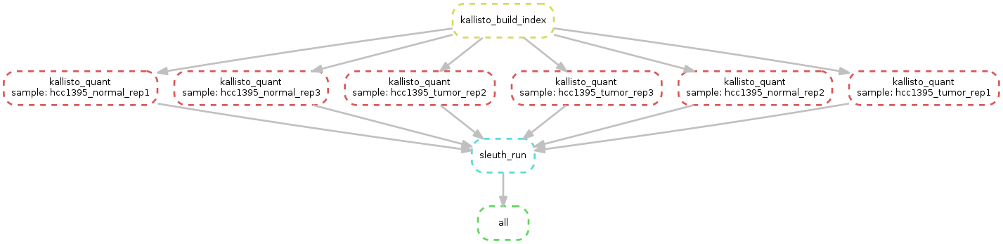
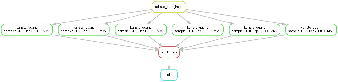
Practical 1 (Kallisto->Sleuth->Shiny)

In this session we want to perform differential expression using pseudomapping approach from kallisto and Sleuth for call differential expression genes. Sleuth makes use of quantification uncertainty estimates obtained via kallisto for accurate differential analysis of isoforms or genes, allows testing in the context of experiments with complex designs, and supports interactive exploratory data analysis via sleuth livesleuth. For this analisys I wrote pipeline using Snakemake [Snakemake] (https://snakemake.readthedocs.io/en/stable/). Please try to do index using kallisto and pseudomap; after that use sleuth.

The test data consists of two commercially available RNA samples: Universal Human Reference (UHR) and Human Brain Reference (HBR). The UHR is total RNA isolated from a diverse set of 10 cancer cell lines. The HBR is total RNA isolated from the brains of 23 Caucasians, male and female, of varying age but mostly 60-80 years old. In addition, a spike-in control was used. Specifically we added an aliquot of the ERCC ExFold RNA Spike-In Control Mixes to each sample. The spike-in consists of 92 transcripts that are present in known concentrations across a wide abundance range (from very few copies to many copies). This range allows us to test the degree to which the RNA-seq assay (including all laboratory and analysis steps) accurately reflects the relative abundance of transcript species within a sample. There are two ‘mixes’ of these transcripts to allow an assessment of differential expression output between samples if you put one mix in each of your two comparisons. In our case, Mix1 was added to the UHR sample, and Mix2 was added to the HBR sample. We also have 3 complete experimental replicates for each sample. This allows us to assess the technical variability of our overall process of producing RNA-seq data in the lab.

So to summarize we have:

    UHR + ERCC Spike-In Mix1, Replicate 1
    UHR + ERCC Spike-In Mix1, Replicate 2
    UHR + ERCC Spike-In Mix1, Replicate 3
    HBR + ERCC Spike-In Mix2, Replicate 1
    HBR + ERCC Spike-In Mix2, Replicate 2
    HBR + ERCC Spike-In Mix2, Replicate 3

Each data set has a corresponding pair of FastQ files (read 1 and read 2 of paired end reads). The reads are paired-end 101-mers generated on an Illumina HiSeq instrument. The test data has been pre-filtered for reads that appear to map to chromosome 22. Lets copy the raw input data to our tutorial working directory.(This data are online avaible from the tutorial course of Malachi Greiffith [link](https://github.com/griffithlab/rnaseq_tutorial/wiki(.

Please downlad the material here: data

What we want to do is this: - Index the reference - Map using kallisto - Use Sleuth for differential expression - Use Sleuth live

Please follow this command

cd ~/Desktop/
mv ~/Download/RNA_kallisto2.tar.bzip2
cd RNA_kallisto2/
ls -ltr 
zcat RAW/UHR_Rep1_ERCC-Mix1_Build37-ErccTranscripts-chr22.read1.fastq.gz | head -n 8
conda env create -f snakemake_differential.yml
source activate snakemake
snakemake -s Snakemake.kallisto --configfile database3.yaml --use-conda 

Please launch the analysis:

snakemake -s Snakefile.Kallisto --configfile database3.yml --use-conda

when finish see the results and open Rstudio:

       install.packages("devtools")
       devtools::install_github("pachterlab/sleuth")
       library("sleuth")
      load(file="kallisto/DEGS/sleuth_object.RData")
      sleuth_live(so)


        <img src="https://bioinfo-dirty-jobs.github.io/master_course//images/02.01.png" >

Chech the tools present

   <img src="https://bioinfo-dirty-jobs.github.io/master_course//images/2.sleuthshini2.png" >

Check the PCA

Please Connect and see this tutorial on live sleuth

[youtube](https://www.youtube.com/watch?v=KEn0CMYk6Wo)
[blog](https://liorpachter.wordpress.com/2015/08/17/a-sleuth-for-rna-seq/)
[another_tutorial](https://pachterlab.github.io/sleuth_walkthroughs/trapnell/analysis.html)

PRACTICAL COUNTS DATA

In the previous example we use the new way to do RNA-seq analisys using pseudomap approach. This method are recently reported (Kallisto and Salmon). Another way to do this type analisys was performed using counts. Normally you can allign with programs like STAR and count gene and isoforms using HTseq-count or feature-count. Here we are some examples of working on R on Counts.

Please open R-studio

And install airway package from bioconductor airway This package provides a RangedSummarizedExperiment object of read counts in genes for an RNA-Seq experiment on four human airway smooth muscle cell lines treated with dexamethasone. Details on the gene model and read counting procedure are provided in the package vignette.

    ### Experimental data
    The data used in this workflow is stored in the airway package that summarizes an RNA-seq experiment wherein airway smooth muscle cells were treated with dexamethasone, a synthetic glucocorticoid steroid with anti-inflammatory effects (Himes et al. 2014). Glucocorticoids are used, for example, by people with asthma to reduce inflammation of the airways. In the experiment, four primary human airway smooth muscle cell lines were treated with 1 micromolar dexamethasone for 18 hours. For each of the four cell lines, we have a treated and an untreated sample. For more description of the experiment see the PubMed entry 24926665 and for raw data see the GEO entry GSE52778.

source("https://bioconductor.org/biocLite.R")
biocLite("airway")

Then activate DESEQ2 and star to read the vignette DESEq2

  library("airway")
  indir <- system.file("extdata", package="airway", mustWork=TRUE)
  list.files(indir) We now use R’s data command to load a prepared SummarizedExperiment that was generated from the publicly available sequencing data files associated with Himes et al. (2014), described above. The steps we used to produce this object were equivalent to those you worked through in the previous sections, except that we used all the reads and all the genes. For more details on the exact steps used to create this object, type vignette("airway") into your R session.

        data("airway")
        se <- airway

  ## ------------------------------------------------------------------------
  se$dex %<>% relevel("untrt")
  se$dex

  ## ------------------------------------------------------------------------
  round( colSums(assay(se)) / 1e6, 1 )

  ## ------------------------------------------------------------------------
  colData(se)

  ## ------------------------------------------------------------------------
  library("DESeq2")

  ## ------------------------------------------------------------------------
  dds <- DESeqDataSet(se, design = ~ cell + dex)

  ## ------------------------------------------------------------------------
  countdata <- assay(se)
  head(countdata, 3)

  ## ------------------------------------------------------------------------
  coldata <- colData(se)

  ## ------------------------------------------------------------------------
  ddsMat <- DESeqDataSetFromMatrix(countData = countdata,
                                    colData = coldata,
                                    design = ~ cell + dex)

  ## ------------------------------------------------------------------------
  nrow(dds)
  dds <- dds[ rowSums(counts(dds)) > 1, ]
  nrow(dds)

  ## ----meanSdCts-----------------------------------------------------------
  lambda <- 10^seq(from = -1, to = 2, length = 1000)
  cts <- matrix(rpois(1000*100, lambda), ncol = 100)
  library("vsn")
  meanSdPlot(cts, ranks = FALSE)

  ## ----meanSdLogCts--------------------------------------------------------
  log.cts.one <- log2(cts + 1)
  meanSdPlot(log.cts.one, ranks = FALSE)

  ## ----rlog----------------------------------------------------------------
  rld <- rlog(dds, blind = FALSE)
  head(assay(rld), 3)

  ## ----vst-----------------------------------------------------------------
  vsd <- vst(dds, blind = FALSE)
  head(assay(vsd), 3)

  ## ----rldplot, fig.width = 6, fig.height = 2.5----------------------------
  library("dplyr")
  library("ggplot2")

  dds <- estimateSizeFactors(dds)

  df <- bind_rows(
    as_data_frame(log2(counts(dds, normalized=TRUE)[, 1:2]+1)) %>%
           mutate(transformation = "log2(x + 1)"),
    as_data_frame(assay(rld)[, 1:2]) %>% mutate(transformation = "rlog"),
    as_data_frame(assay(vsd)[, 1:2]) %>% mutate(transformation = "vst"))
    
  colnames(df)[1:2] <- c("x", "y")  

  ggplot(df, aes(x = x, y = y)) + geom_hex(bins = 80) +
    coord_fixed() + facet_grid( . ~ transformation)  

  ## ------------------------------------------------------------------------
  sampleDists <- dist(t(assay(rld)))
  sampleDists

  ## ------------------------------------------------------------------------
  library("pheatmap")
  library("RColorBrewer")

  ## ----distheatmap, fig.width = 6.1, fig.height = 4.5----------------------
  sampleDistMatrix <- as.matrix( sampleDists )
  rownames(sampleDistMatrix) <- paste( rld$dex, rld$cell, sep = " - " )
  colnames(sampleDistMatrix) <- NULL
  colors <- colorRampPalette( rev(brewer.pal(9, "Blues")) )(255)
  pheatmap(sampleDistMatrix,
           clustering_distance_rows = sampleDists,
           clustering_distance_cols = sampleDists,
           col = colors)

  ## ------------------------------------------------------------------------
  library("PoiClaClu")
  poisd <- PoissonDistance(t(counts(dds)))

  ## ----poisdistheatmap, fig.width = 6.1, fig.height = 4.5------------------
  samplePoisDistMatrix <- as.matrix( poisd$dd )
  rownames(samplePoisDistMatrix) <- paste( rld$dex, rld$cell, sep=" - " )
  colnames(samplePoisDistMatrix) <- NULL
  pheatmap(samplePoisDistMatrix,
           clustering_distance_rows = poisd$dd,
           clustering_distance_cols = poisd$dd,
           col = colors)

  ## ----plotpca, fig.width=6, fig.height=4.5--------------------------------
  plotPCA(rld, intgroup = c("dex", "cell"))

  ## ------------------------------------------------------------------------
  pcaData <- plotPCA(rld, intgroup = c( "dex", "cell"), returnData = TRUE)
  pcaData
  percentVar <- round(100 * attr(pcaData, "percentVar"))

  ## ----ggplotpca, fig.width=6, fig.height=4.5------------------------------
  ggplot(pcaData, aes(x = PC1, y = PC2, color = dex, shape = cell)) +
    geom_point(size =3) +
    xlab(paste0("PC1: ", percentVar[1], "% variance")) +
    ylab(paste0("PC2: ", percentVar[2], "% variance")) +
    coord_fixed()

  ## ----mdsrlog, fig.width=6, fig.height=4.5--------------------------------
  mds <- as.data.frame(colData(rld))  %>%
           cbind(cmdscale(sampleDistMatrix))
  ggplot(mds, aes(x = `1`, y = `2`, color = dex, shape = cell)) +
    geom_point(size = 3) + coord_fixed()

  ## ----mdspois, fig.width=6, fig.height=4.5--------------------------------
  mdsPois <- as.data.frame(colData(dds)) %>%
     cbind(cmdscale(samplePoisDistMatrix))
  ggplot(mdsPois, aes(x = `1`, y = `2`, color = dex, shape = cell)) +
    geom_point(size = 3) + coord_fixed()

  ## ----airwayDE------------------------------------------------------------
  dds <- DESeq(dds)

  ## ------------------------------------------------------------------------
  res <- results(dds)
  res

  ## ------------------------------------------------------------------------
  res <- results(dds, contrast=c("dex","trt","untrt"))

  ## ------------------------------------------------------------------------
  mcols(res, use.names = TRUE)

  ## ------------------------------------------------------------------------
  summary(res)

  ## ------------------------------------------------------------------------
  res.05 <- results(dds, alpha = 0.05)
  table(res.05$padj < 0.05)

  ## ------------------------------------------------------------------------
  resLFC1 <- results(dds, lfcThreshold=1)
  table(resLFC1$padj < 0.1)

  ## ------------------------------------------------------------------------
  results(dds, contrast = c("cell", "N061011", "N61311"))

  ## ----sumres--------------------------------------------------------------
  sum(res$pvalue < 0.05, na.rm=TRUE)
  sum(!is.na(res$pvalue))

  ## ------------------------------------------------------------------------
  sum(res$padj < 0.1, na.rm=TRUE)

  ## ------------------------------------------------------------------------
  resSig <- subset(res, padj < 0.1)
  head(resSig[ order(resSig$log2FoldChange), ])

  ## ------------------------------------------------------------------------
  head(resSig[ order(resSig$log2FoldChange, decreasing = TRUE), ])

  ## ----plotcounts----------------------------------------------------------
  topGene <- rownames(res)[which.min(res$padj)]
  plotCounts(dds, gene = topGene, intgroup=c("dex"))

  ## ----ggplotcountsjitter, fig.width = 4, fig.height = 3-------------------
  library("ggbeeswarm")
  geneCounts <- plotCounts(dds, gene = topGene, intgroup = c("dex","cell"),
                           returnData = TRUE)
  ggplot(geneCounts, aes(x = dex, y = count, color = cell)) +
    scale_y_log10() +  geom_beeswarm(cex = 3)

  ## ----ggplotcountsgroup, fig.width = 4, fig.height = 3--------------------
  ggplot(geneCounts, aes(x = dex, y = count, color = cell, group = cell)) +
    scale_y_log10() + geom_point(size = 3) + geom_line()

  ## ----plotma--------------------------------------------------------------
  res <- lfcShrink(dds, contrast=c("dex","trt","untrt"), res=res)
  plotMA(res, ylim = c(-5, 5))

  ## ----plotmaNoShr---------------------------------------------------------
  res.noshr <- results(dds)
  plotMA(res.noshr, ylim = c(-5, 5))

  ## ----plotmalabel---------------------------------------------------------
  plotMA(res, ylim = c(-5,5))
  topGene <- rownames(res)[which.min(res$padj)]
  with(res[topGene, ], {
    points(baseMean, log2FoldChange, col="dodgerblue", cex=2, lwd=2)
    text(baseMean, log2FoldChange, topGene, pos=2, col="dodgerblue")
  })

  ## ----histpvalue2---------------------------------------------------------
  hist(res$pvalue[res$baseMean > 1], breaks = 0:20/20,
       col = "grey50", border = "white")

  ## ------------------------------------------------------------------------
  library("genefilter")
  topVarGenes <- head(order(rowVars(assay(rld)), decreasing = TRUE), 20)

  ## ----genescluster--------------------------------------------------------
  mat  <- assay(rld)[ topVarGenes, ]
  mat  <- mat - rowMeans(mat)
  anno <- as.data.frame(colData(rld)[, c("cell","dex")])
  pheatmap(mat, annotation_col = anno)

  ## ----sensitivityovermean, fig.width=6------------------------------------
  qs <- c(0, quantile(resLFC1$baseMean[resLFC1$baseMean > 0], 0:6/6))
  bins <- cut(resLFC1$baseMean, qs)
  levels(bins) <- paste0("~", round(signif((qs[-1] + qs[-length(qs)])/2, 2)))
  fractionSig <- tapply(resLFC1$pvalue, bins, function(p)
                            mean(p < .05, na.rm = TRUE))
  barplot(fractionSig, xlab = "mean normalized count",
                       ylab = "fraction of small p values")

  ## ------------------------------------------------------------------------
  library("AnnotationDbi")
  library("org.Hs.eg.db")

  ## ------------------------------------------------------------------------
  columns(org.Hs.eg.db)

  ## ------------------------------------------------------------------------
  res$symbol <- mapIds(org.Hs.eg.db,
                       keys=row.names(res),
                       column="SYMBOL",
                       keytype="ENSEMBL",
                       multiVals="first")
  res$entrez <- mapIds(org.Hs.eg.db,
                       keys=row.names(res),
                       column="ENTREZID",
                       keytype="ENSEMBL",
                       multiVals="first")

  ## ------------------------------------------------------------------------
  resOrdered <- res[order(res$pvalue),]
  head(resOrdered)

  ## ----eval=FALSE----------------------------------------------------------
  ## resOrderedDF <- as.data.frame(resOrdered)[1:100, ]
  ## write.csv(resOrderedDF, file = "results.csv")

well DONE!!!

If you want to perform all the tutorial plase make ths step :

    source("http://bioconductor.org/workflows.R")
    workflowInstall("rnaseqGene")

and follow this examples link

SALMON AND SHINY

Please use this data data and follow the snakemake.

    ## List dependencies
    pkg <- c("shiny", "ggplot2", "ggrepel", "dplyr", "tidyr", "Gviz", 
             "DT", "shinydashboard", "GenomicRanges", "IRanges", 
             "rtracklayer", "S4Vectors", "GenomeInfoDb", 
             "BiocGenerics", "devtools")

    ## Check if dependencies are already installed
    pkg <- pkg[!(pkg %in% installed.packages()[, "Package"])]

    ## If some dependency is missing, install it
    if (length(pkg) > 0) {
      source("https://bioconductor.org/biocLite.R")
      biocLite(pkg, dependencies = TRUE, ask = FALSE)
    }

    ## Install iResViewer
    devtools::install_github("csoneson/iResViewer")

OPTIONAL PRATICAL