RNA-seq part 2 DESeq2

RNA-seq data analyss Count

Pipeline

Introduction

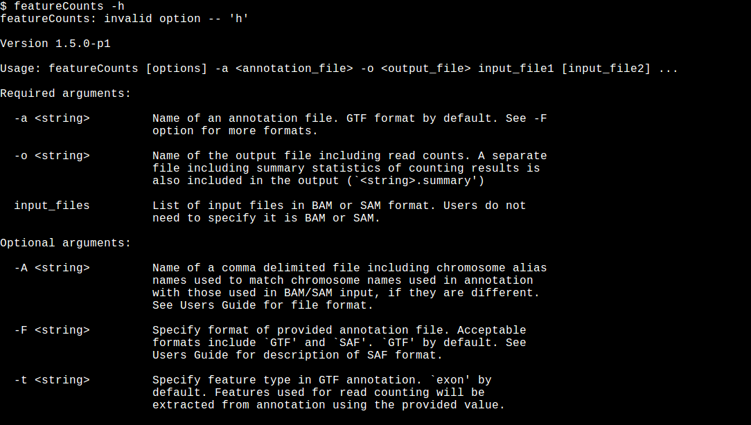
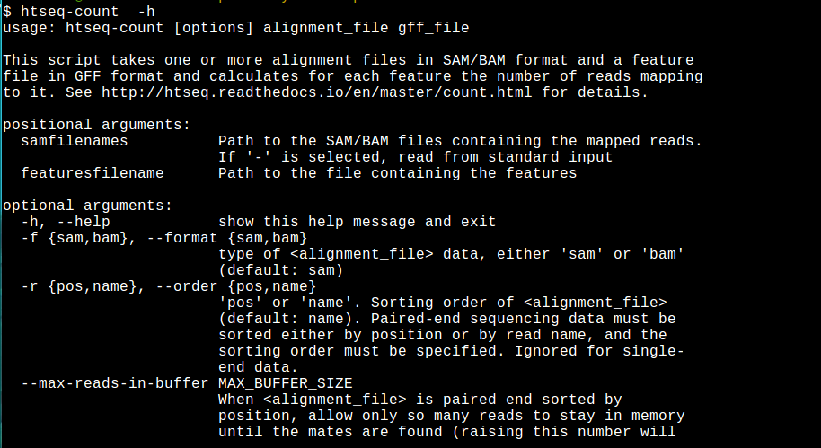
RNA-Seq (RNA sequencing ) also called whole transcriptome sequncing use next-generation sequeincing (NGS) to reveal the presence and quantity of RNA in a biolgical sample at a given moment. As we discuss during the talk we can use different approach and different tools. Here we present the DEseq2 vignette it wwas composed using STAR and HTseqcount and then Deseq2. The other part we show kallisto Unfortunately our computer not allow the work some step was only for demonstration purpose.

Practical 1

RNA-seq workflow: gene-level exploratory analysis and differential expression:

R practical:

Here we are some examples of working on R on Counts.

For count

We can use R

    conda create -n DESEQ
    source activate DESEQ
      conda install -y r-mixomics  bioconductor-htsfilter bioconductor-deseq2
    R
  library(DESeq2)
  library(RColorBrewer)
  library(mixOmics)
  library(HTSFilter) 
  
directory <- "RNAseq_data/count_table_files/"
dir(directory)

*Exercise 3.1* Read the files:

rawCountTable <- read.table(paste0(directory,"count_table.tsv"), header=TRUE,
                            row.names=1)
sampleInfo <- read.table(paste0(directory,"pasilla_design.txt"), header=TRUE,
                         row.names=1)

*Exercise 3.2* Have a look at the count data:
head(rawCountTable)
nrow(rawCountTable)

*Exercise 3.3* Have a look at the sample information and order the count table
in the same way that the sample information:
sampleInfo
rawCountTable <- rawCountTable[,match(rownames(sampleInfo),
                                      colnames(rawCountTable))]
head(rawCountTable)

*Exercise 3.4* Create the 'condition' column
sampleInfo$condition <- substr(rownames(sampleInfo), 1,
                               nchar(rownames(sampleInfo))-1)
sampleInfo$condition[sampleInfo$condition=="untreated"] <- "control"
sampleInfo$condition <- factor(sampleInfo$condition)
sampleInfo

*Exercise 3.5* Create a 'DESeqDataSet' object
ddsFull <- DESeqDataSetFromMatrix(as.matrix(rawCountTable), sampleInfo,
                                  formula(~condition))
ddsFull

# 3.2. Starting from separate files

*Exercise 3.6* List all files in directory

directory <- "RNAseq_data/separate_files/"
sampleFiles <- list.files(directory)
sampleFiles

*Exercise 3.7* Create an object with file informations

keptFiles <- sampleFiles[-1]
sampleName <- sapply(keptFiles, function(afile)
  substr(afile, 1, nchar(afile)-6))
condition<- sapply(keptFiles, function(afile) 
  substr(afile, 1, nchar(afile)-7))
fileInfo <- data.frame(sampleName = sampleName, sampleFiles = keptFiles,
                       condition = condition)
rownames(fileInfo) <- NULL
fileInfo

*Exercise 3.8* Construct a 'DESeqDataSet' object

ddsHTSeq <- DESeqDataSetFromHTSeqCount(fileInfo, directory, formula(~condition))
ddsHTSeq

# 3.3. Preparing the data object for the analysis of interest

*Exercise 3.9* Select the subset of paire-end samples
dds <- subset(ddsFull, select=colData(ddsFull)$type=="paired-end")
dds
colData(dds)

# 3.4 Data exploration and quality assessment

*Exercise 3.10* Extract pseudo-counts (*ie* $\log_2(K+1)$) 
pseudoCounts <- log2(counts(dds)+1)
head(pseudoCounts)
*Exercise 3.11* Histogram for pseudo-counts (sample ```treated2```)
```{r histoPseudoCounts}
hist(pseudoCounts[,"treated2"])

*Exercise 3.12* Boxplot for pseudo-counts
boxplot(pseudoCounts, col="gray")

*Exercise 3.13* MA-plots between control or treated samples
par(mfrow=c(1,2))
## treated2 vs treated3
# A values
avalues <- (pseudoCounts[,1] + pseudoCounts[,2])/2
# M values
mvalues <- (pseudoCounts[,1] - pseudoCounts[,2])
plot(avalues, mvalues, xlab="A", ylab="M", pch=19, main="treated")
abline(h=0, col="red")
## untreated3 vs untreated4
# A values
avalues <- (pseudoCounts[,3] + pseudoCounts[,4])/2
# M values
mvalues <- (pseudoCounts[,3] - pseudoCounts[,4])
plot(avalues, mvalues, xlab="A", ylab="M", pch=19, main="control")
abline(h=0, col="red")

*Exercise 3.14* PCA for pseudo-counts
vsd <- varianceStabilizingTransformation(dds)
vsd
plotPCA(vsd)

*Exercise 3.15* heatmap for pseudo-counts (using ```mixOmics``` package)
sampleDists <- as.matrix(dist(t(pseudoCounts)))
sampleDists
cimColor <- colorRampPalette(rev(brewer.pal(9, "Blues")))(16)
cim(sampleDists, col=cimColor, symkey=FALSE)

# 3.5. Differential expression analysis

*Exercise 3.16* Run the DESeq2 analysis
dds <- DESeq(dds)
dds

# 3.6. Inspecting the results

*Exercise 3.17* Extract the results
res <- results(dds)
res

*Exercise 3.18* Obtain information on the meaning of the columns
mcols(res)

*Exercise 3.19* Count the number of significant genes at level 1%
sum(res$padj < 0.01, na.rm=TRUE)

*Exercise 3.20* Extract significant genes and sort them by the strongest down
regulation
sigDownReg <- res[!is.na(res$padj), ]
sigDownReg <- sigDownReg[sigDownReg$padj < 0.01, ]
sigDownReg <- sigDownReg[order(sigDownReg$log2FoldChange),]
sigDownReg

*Exercise 3.21* Extract significant genes and sort them by the strongest up
regulation
sigUpReg <- res[!is.na(res$padj), ]
sigUpReg <- sigUpReg[sigUpReg$padj < 0.01, ]
sigUpReg <- sigUpReg[order(sigUpReg$log2FoldChange, decreasing=TRUE),]
*Exercise 3.22* Create permanent storage of results
write.csv(sigDownReg, file="sigDownReg-deseq.csv")
write.csv(sigUpReg, file="sigUpReg-deseq.csv")

# 3.7 Diagnostic plot for multiple testing

*Exercise 3.23* Plot a histogram of unadjusted p-values after filtering
hist(res$pvalue, breaks=50)

# 3.8 Interpreting the DE analysis results

*Exercise 3.24* Create a MA plot showing differentially expressed genes
plotMA(res, alpha=0.01)

*Exercise 3.25* Create a Volcano plot
volcanoData <- cbind(res$log2FoldChange, -log10(res$padj))
volcanoData <- na.omit(volcanoData)
colnames(volcanoData) <- c("logFC", "negLogPval")
head(volcanoData)
plot(volcanoData, pch=19, cex=0.5)

*Exercise 3.26* Transform the normalized counts for variance stabilization
vsnd <- varianceStabilizingTransformation(dds, blind=FALSE)
vsnd

*Exercise 3.27* Extract the transformed data
head(assay(vsnd), 10)
selY <- assay(vsnd)[!is.na(res$pval), ]
selY <- selY[res$pval[!is.na(res$pval)] < 0.01,]
cimColor <- colorRampPalette(rev(brewer.pal(9, "Blues")))(255)[255:1]
cim(t(selY), col=cimColor, symkey=FALSE)

Practical 2

In this session we want to perform some differential expression from two conditions as example (Normal vs tumor RNA-seq). This data use for this tutorial are pubblicaly avaible.

Please download the material here:

Kallisto tutorial

Please follow this command

    cd ~/Desktop/
    tar xvf TUTORIAL_RNA_snakemake.tar.gz
    cd TUTORIAL
    conda env create -f snakemake_differential.yml
    

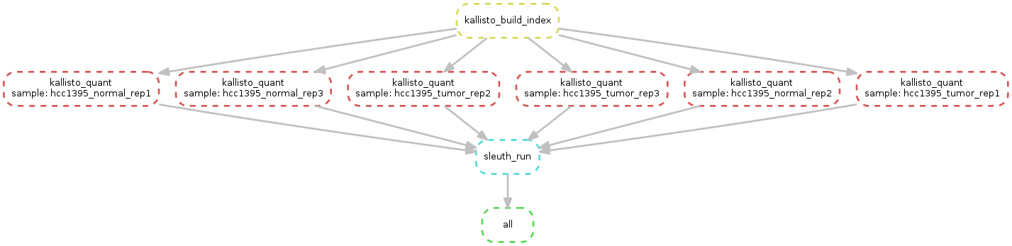
Please launch the analysis in this way:


    snakemake -s Snakefile.Kallisto --configfile database3.yml --use-conda

Please Connect and see this tutorial on live sleuth:

[youtube](https://www.youtube.com/watch?v=KEn0CMYk6Wo)

KALLISTO PIPELINE USING NEXTFLOW

Here antoher way to do the analysis. Please familiarize with the results

  cd  /home/bioinfo2/Data/kallisto-nf 
  sudo nextflow run cbcrg/kallisto-nf -with-docker

OPTIONAL PRATICAL

Please follow this tutorial [link] (http://www.nathalievilla.org/doc/html/solution_edgeR-tomato.html#where-to-start-installation-and-alike) Pratical rnaseq data using tomato data